Adventures into Natural Language Processing

Summary

The capstone project consists of applying data science in the area of natural language processing. The data, a collection of text documents also known as corpus, have been collected from different webpages and different types of sources. In particular, for this project, we analyze corpora in american english from three distinct sources: twitter, blogs and news media sites. The files have been language filtered but may still contain some foreign text. Below, we report the major features of the data that have been identified and we briefly summarize the plans for creating a prediction algorithm.

Data Exploration

The data consists of three different collection of texts or corpora, en_US.blogs.txt taken from blogs, en_US.news.txt from news sites and en_US.twitter.txt from twitter. In the following we will refer to these datafiles or corpora simply by its source, i.e. blogs, news and twitter. The following table presents word and line count for each of the three corpora.

data <- data.frame(c('en_US.blogs.txt','en_US.news.txt','en_US.twitter.txt'),
                   c('899,288','1,010,242','2,360,148'),
                   c('37,334,690','34,372,720','30,374,206'))
names(data) <- c("corpus","lines","words")
library(knitr)
#library(xtable)
kable(data,align='c',padding=0,digits=1)

We use the tm framework for cleaning the documents and the RWeka package for tokenization. Given the sheer amount of data contained in the three corpora, the analysis is performed in a random sample of approximately 1% of the total data.

path <- '~/Documents/coursera/datasciencecoursera/capstone/data/final/en_US/'
setwd(path)
library(tm)
library(RWeka)
require(NLP)
options(mc.cores=1) # to avoid possible conflicts of the RWeka package.

In the process of cleaning and preprocessing the data, the following transformations were performed:

each word was converted to lower-case, e.g. Tree to tree
removal of URLs, e.g. www.someaddress.com
removal of punctuation: commas, colons, semicolons, dashes, parentheses
removal of numbers
removal of stopwords, such as a, the, to, etc.

mycorpus <- function(file,lines){
    con <- file(file,'r')
    txt <- readLines(con,lines)
    close(con)
    
    removeURL <- function(x) gsub("http[[:alnum:]]*", "", x)
    removeWWW <- function(x) gsub("www[[:alnum:]]*", "", x)
    
    #load corpus from text source
    corpus <- VCorpus(VectorSource(txt))
    
    # clean corpus
    corpus <- tm_map(corpus, content_transformer(tolower)) #lower case    
    corpus <- tm_map(corpus, content_transformer(removeURL))
    corpus <- tm_map(corpus, content_transformer(removeWWW))
    corpus <- tm_map(corpus, removePunctuation)
    corpus <- tm_map(corpus, removeNumbers)
    corpus <- tm_map(corpus, removeWords, stopwords("english"))
    corpus <- tm_map(corpus, stripWhitespace)
    corpus
}

n <- 7000; n2 <- 18000
blogs.corpus <- mycorpus(paste0(path,'en_US.blogs.txt'),5500)
news.corpus <- mycorpus(paste0(path,'en_US.news.txt'),n)
twitter.corpus <- mycorpus(paste0(path,'en_US.twitter.txt'),n2)

# term-document matrix function
tokens <- function(corpus){
    dtm <- DocumentTermMatrix(corpus)
    tokens <- sort(apply(dtm,2,sum),decreasing = TRUE)
    freq.words <- findFreqTerms(dtm,10)
    returnlist <- list(tokens,freq.words)
    returnlist
}

alist <- tokens(blogs.corpus)
tokens.blogs <- alist[[1]]
freq.words.blogs <- alist[[2]]

alist <- tokens(news.corpus)
tokens.news <- alist[[1]]
freq.words.news <- alist[[2]]

alist <- tokens(twitter.corpus)
tokens.twitter <- alist[[1]]
freq.words.twitter <- alist[[2]]

After cleaning and processing the text databases, the number of unique words is as follows:

corp<-c('en_US.news.txt','en_US.twitter.txt','en_US.blogs.txt')
lu<-c(length(tokens.news),length(tokens.twitter),length(tokens.blogs))
lt<-c(sum(tokens.news),sum(tokens.twitter),sum(tokens.blogs))
d <- data.frame(corp,lu,lt)
names(d) <- c('corpus','unique words','total words')

kable(d,align = 'c')

Below we show the top ten most frequent words for each of the corpora.

par(mfrow=c(1,3))
barplot(tokens.blogs[1:10],
      #  xlab='token',
        ylab='frequency',
        main='en_US.blogs.txt',
        names.arg=names(tokens.blogs)[1:10],        
        las=2)

barplot(tokens.news[1:10],
      #  xlab='token',
        ylab='frequency',
        main='en_US.news.txt',
        names.arg=names(tokens.news)[1:10],        
        las=2)

barplot(tokens.twitter[1:10],
       # xlab='token',
        ylab='frequency',
        main='en_US.twitter.txt',
        names.arg=names(tokens.twitter)[1:10],        
        las=2)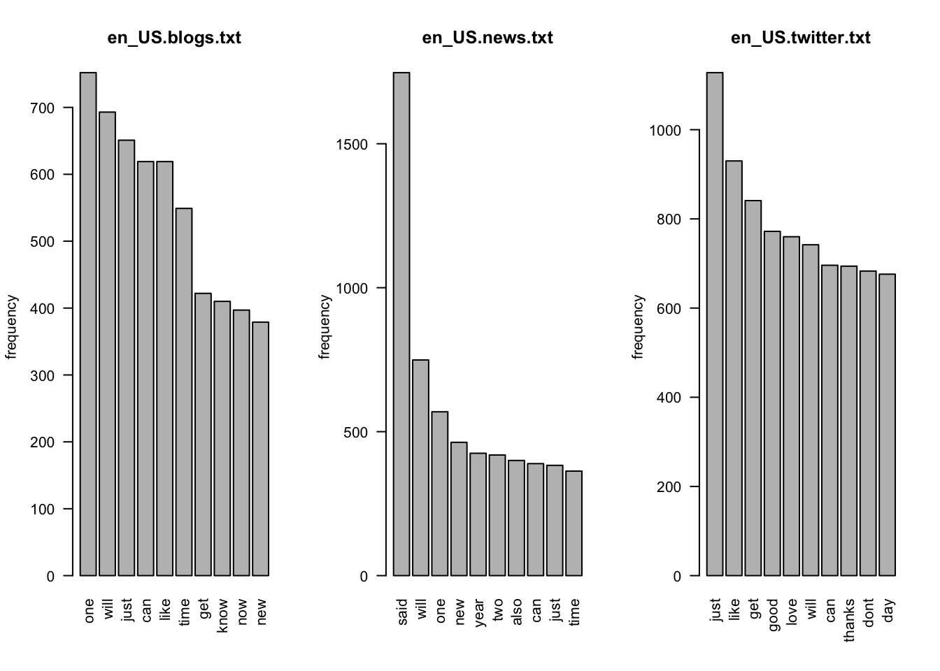

top words per corpus

The number of unique words needed to cover the entire language (sample).

plot(cumsum(tokens.news)/sum(tokens.news),type="l",col="blue",
     xlab="unique words",
     ylab="Percentage of all word")
    # main="Cumulative")
lines(cumsum(tokens.twitter)/sum(tokens.twitter),type="l",col="red")
lines(cumsum(tokens.blogs)/sum(tokens.blogs),type="l",col="green")
legend("bottomright",legend = c("news","twitter","blogs"),
       col=c("blue","red","green"),lwd=1)

#tokenization
#word.tokens <- WordTokenizer()
# word frequency
# profanity filtering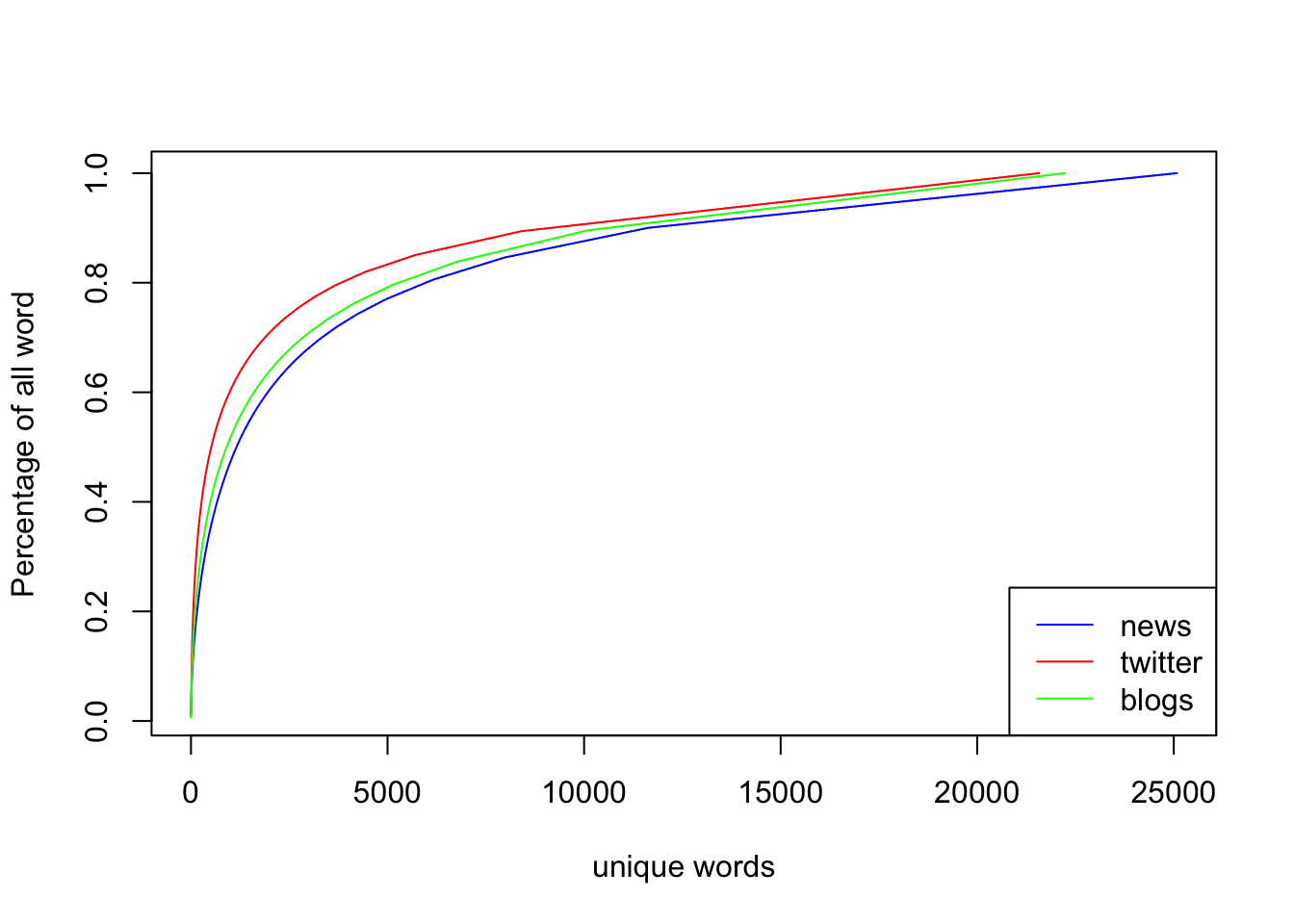

unique word coverage

To aquire acceptable accuracy of the prediction algorithm, it is important to obtain the frequency of pair of words or bigrams. Accuracy is improved by further incorporating into the model frequencies of longer word sequences, three-, four- or n-grams.

# bi-grams
getBigrams <- function(x) RWeka::NGramTokenizer(x, Weka_control(min=2,max=2))
#getTrigrams <-function(x) NGramTokenizer(x, Weka_control(min=3,max=3))
bidtm.blogs <- DocumentTermMatrix(blogs.corpus,control=list(tokenize=getBigrams))

bidtm.news <- DocumentTermMatrix(news.corpus,control=list(tokenize=getBigrams))

bidtm.twitter <- DocumentTermMatrix(twitter.corpus,control=list(tokenize=getBigrams))
#trigrambag <- DocumentTermMatrix(blogs.corpus,control=list(tokenize=getTrigrams))

bigrams.blogs <- sort(apply(bidtm.blogs,2,sum),decreasing = TRUE)
bigrams.news <- sort(apply(bidtm.news,2,sum),decreasing = TRUE)
bigrams.twitter <- sort(apply(bidtm.twitter,2,sum),decreasing = TRUE)

#bigrams.news[1:10]
#bigrams.twitter[1:10]
#bigrams.blogs[1:10]
par(mfrow=c(1,2))
barplot(bigrams.news[1:5],
       # xlab='token',
        ylab='frequency',
        main='en_US.news.txt',
        names.arg=names(bigrams.news)[1:5],        
        las=2)

barplot(bigrams.twitter[1:5],
     #   xlab='token',
        ylab='frequency',
        main='en_US.twitter.txt',
        names.arg=names(bigrams.twitter)[1:5],        
        las=2)

#barplot(bigrams.blogs[1:10],
     #   xlab='token',
 #       ylab='frequency',
 #       main='Most Frequent Bigrams in en_US.blogs.txt',
 #       names.arg=names(bigrams.blogs)[1:10],        
 #       las=2)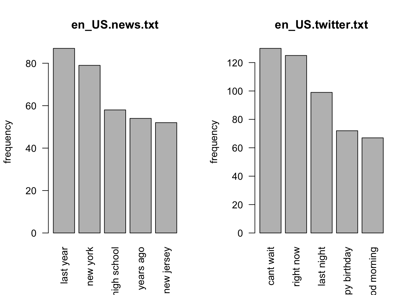

Discussion

There are subtle differences in the three databases. Therefore it seems that the optimal prediction algorithm would contain a weighted average of the n-grams obtained from the three sources at our disposal. Accuracy can be improved as well with more detailed cleaning of the data and by adjusting the processing according to the type of source of the data. Stop words will be included back to be able to predict without adding too much complexity to the prediction algorithm.